Supervised PCA transform.

txSpca transforms data using supervised principal component analysis. TODO

txSpca(x, y = diag(1, nrow(x)), k = 3, ...)

Arguments

x	a data matrix (features in columns, samples in rows)
y	target classification of x (logical, numeric, or a factor), or a kernel matrix of the target. If not specified, it defaults to identity matrix, in which case SPCA becomes equivalent to classical PCA (as the matrix being decomposed equals the covariance matrix of 'x'. (Strictly speaking, when centering is in use, SPCA becomes the classical PCA. Otherwise, SPCA yields components similar to those yielded by PCA over centered data, but shifted.)
k	number of dimensions of the result, defaults to 3 in order to be usable in 'plot3dProj'
...	additional arguments to 'spca'

Value

Transform function taking two arguments: a data matrix y to transform, and a logical center determining whether the data are to be centered, or not. The parameters of the transform get returned in the params attribute (see spca). In addition, there is the varExplained function added to the parameters, which takes k, the number of components, and returns the contribution of individual dimensions to the top k components.

See also

spca, txPca, plot3dProj

Examples

tx<-txSpca(iris[,1:4],iris$Species)
plot(tx(iris[1:10,1:4])[,1:2])

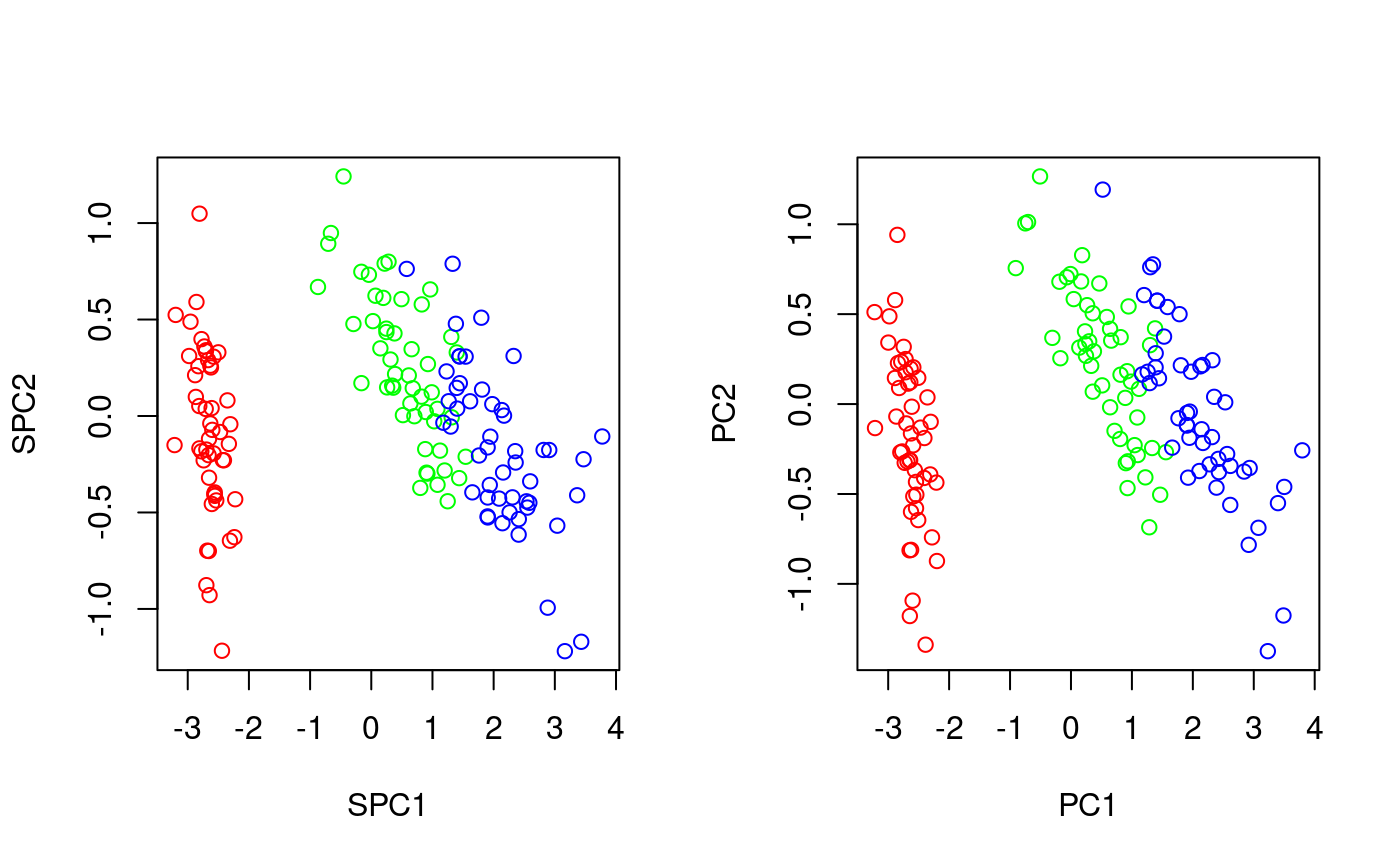
# comparison of PCA vs. SPCA
# TODO
opar<-par(mfrow=c(1,2))
plot(txSpca(iris[,1:4],iris$Species)(iris[,1:4])[,1:2],col=c('red','green','blue')[as.numeric(iris$Species)])
plot(txPca(iris[,1:4])(iris[,1:4])[,1:2],col=c('red','green','blue')[as.numeric(iris$Species)])
par(opar)

if (interactive() && require(rgl)) {
  # a 3D example
  x<-iris[,1:4]
  y<-iris$Species
  plot3dProj(x, cls=y, tx=txSpca(x,y))
}